IO Cost & Trade-offs: Choosing Your Index
Concept. Picking an index is a sequence of three questions. Match the workload to a structure. Decide whether the data is sorted by that key. Then read off the IO cost.
Intuition. Hash wins equality. B+Tree wins range scans. LSM (built on SSTables) wins sustained write throughput. Inverted indexes win full-text. Whether the table is physically sorted by the key (clustered vs unclustered) sets the constant in front of those costs.
This page is structured around three questions. Each maps to one section.
-
How do I choose an index? → Pick the right structure for the workload.
-
What if the data is sorted? → A sorted dictionary needs a much smaller index than an unsorted one. That's clustering.
-
What is the cost? → IO chart per access pattern, plus what
O(log N)actually means in practice.
Q1. How do I choose an index?
Three structures cover almost every relational workload. Match the column to the kind of query that's hot:
| Hash index | B+Tree | LSM (on SSTables) | |
|---|---|---|---|
| Lookup | O(1) equality, hash to bucket, read the entry | O(log N) any key, descend root → internal → leaf | Walks tiers (MemTable → L0 → L1+), Bloom-skipped |
Range / ORDER BY |
None, hash scrambles neighbours | Native, leaves are linked left-to-right | Native, merged view across tiers |
| Write cost | Update one bucket (split on overflow) | Random write + occasional rebalance | Append to RAM, sequential flush, background compaction |
| Typical use | Primary keys, caches | General-purpose OLTP | Counters, events, write-heavy analytics |
| Production examples | Redis, Memcached | PostgreSQL, MySQL InnoDB | Bigtable, Cassandra, DynamoDB, RocksDB |
For full-text search across many documents, the right structure is an inverted index (term dictionary plus postings lists). Used heavily in the Spotify case studies later in the module.
Q2. What if the data is sorted?
Sorted data lets the index scale with N (pages), not n (rows). The intuition is a dictionary.
Two dictionaries with the same content (n = 171,476 words spread over N = 1,000 pages). The only difference: one is sorted, the other isn't.
Webster's: sorted dictionary
- Words appear in alphabetical order from "aardvark" to "zyzzyva".
- Index is sparse: one entry per page (first word + page number), so N = 1,000 entries.
- Find "coffee" with one index lookup ("clutch–coffin → page 217"), jump there, scan a few rows.
Index = ~1,000 entries.
RandomWebster's: unsorted dictionary
- Words are scattered randomly across pages.
- Index must be dense: one entry per word, so n = 171,476 entries.
- "coffee" is on page 847. "coffeehouse" is on page 12. Every word needs its own pointer.
Index = ~171,476 entries (170× larger).
The same idea applied to a database table is clustering.
Clustered index
- Table data is physically sorted by the index key.
- Index is sparse (one entry per page).
- Range scans become sequential reads: find the first page, walk forward.
Best for: the access pattern you scan most.
Unclustered index
- Table data is in insert order, not sorted by the index key.
- Index must be dense (one entry per row).
- Range scans pay one IO per matching row, jumping around the table.
All non-primary indexes are usually unclustered.
A table can only be clustered on one set of columns at a time, because the physical sort order can only go one way. Every other index on the same table is unclustered. Production systems sometimes keep multiple copies of the same table, each clustered differently, when several access patterns need to be fast.
Q3. What is the cost?
Pull the structural choice (Q1) and the clustered/unclustered choice (Q2) together, and you get the IO cost for any access pattern.
What "O(log N)" actually means
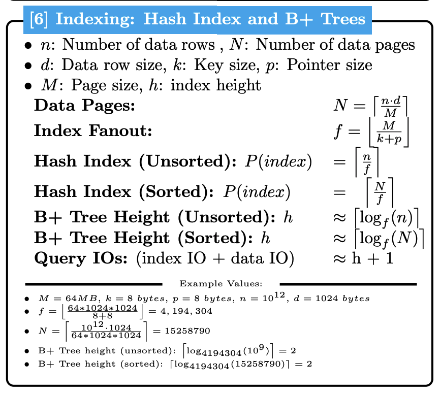
The Big-O hides a lot. A B+Tree's O(log N) is ⌈log_fanout(N)⌉, and fanout is large: at fanout 1,000 a billion-row table fits in just 3 levels, and at fanout 65,000 a trillion-row table fits in 3 levels too. So the asymptotic claim collapses to a constant in practice: roughly 3 to 4 page reads per point lookup, regardless of table size. (See the fanout table on the B+Tree page for the exact arithmetic across page sizes from 64 KB to 64 MB.)
When you compare hash (O(1)) against B+Tree (O(log N)), the real difference is small (1 vs 3 page reads). The useful difference is whether the index supports range scans. The Big-O is asymptotic shorthand, not a recipe for choice.
What drives LSM cost: SSTable counts, not Big-O
LSM costs don't fit cleanly on the asymptotic chart, because they aren't a function of the table size. They're a function of how many SSTables are sitting at each level at the moment you read or write.
-
Reads: walk the MemTable, then every Level-0 SSTable that might contain the key, then the Level-1+ file. The cost is the count of SSTables touched (Bloom-filter-skipped where possible). For a counter, that means summing fragments from each tier. For a latest-wins value, it means returning the first match.
-
Writes: the MemTable buffers writes in RAM. When it fills, sorting it produces one SSTable. That sort is the same in-memory operation as the big sort algorithm. When compaction merges several Level-0 files into one Level-1+ file, that's a sort-merge across already-sorted runs. No new algorithm. Same primitives, applied to LSM's tier structure.
So when you reason about LSM cost, count SSTables and remember which operation is doing the work: in-memory sort for a flush, sort-merge for a compaction.
See also. The big sort page walks through how a runs-and-merge sort actually streams through memory and disk, and the sort-merge join page works the merge step end-to-end. The LSM compaction loop is the same algorithm, with SSTables as the input runs.
Key Insights
-
Three questions, in order. Workload picks the structure. Sorted-or-not picks clustered vs unclustered. The combination tells you the IO cost.
-
O(log N)is asymptotic shorthand. B+Tree point lookups are 3 to 4 IOs, not "growing with table size." The structural fit (range vs equality vs writes) matters more than the asymptote. -
Clustered or unclustered sets the constant. Once you've picked a structure, the physical sort order of the data decides whether range scans are sequential or one-IO-per-row.
Next
Index Problem Solving → Ten concrete scenarios that ask which index type to use and why.