IO Cost Summary: Comparing Query Plans
Concept. The IO cost of a query plan is the sum of the IO costs of every step in the plan. To compare plans, you add up each step's cost using the formulas for sort, hash partition, and the three join algorithms.
Intuition. Two plans that produce the same result can cost wildly different amounts of IO depending on which algorithm you use at each step. This page walks through one recommendation query and computes the total cost of three plausible plans side by side.
The Query
-- Highly recommended songs
SELECT r.song_id, COUNT(r.recommendation_id) AS recommendation_count
FROM Recommendations AS r
JOIN Listens AS l ON r.user_id = l.user_id AND r.song_id = l.song_id
GROUP BY r.song_id
ORDER BY COUNT(r.recommendation_id) DESC;
Three goals to achieve in any plan: JOIN the two tables, GROUP BY song_id, then SORT by count.
Query Plan #1: Sort-Merge Join
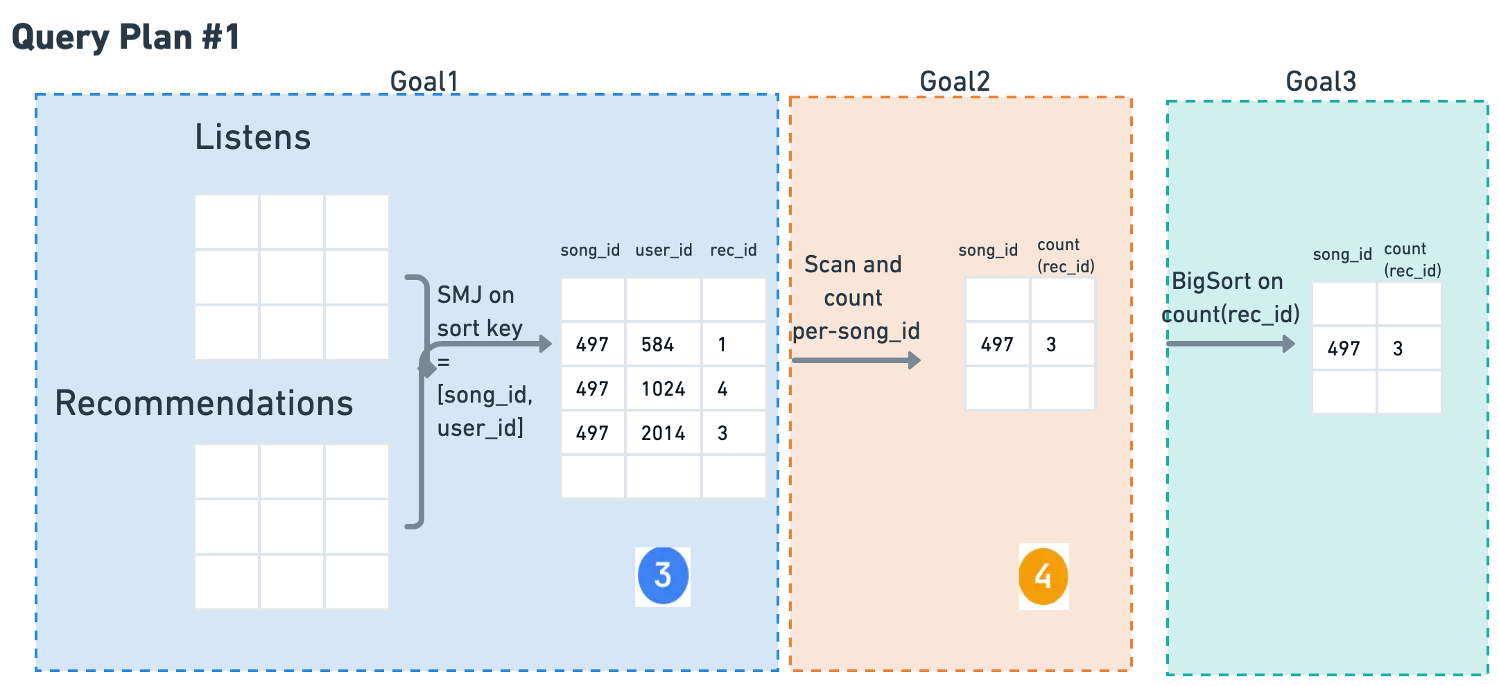
Figure: Plan #1 uses a sort-merge join, which produces already-sorted output we can group directly on `song_id`.
| Goal | What happens | Cost |
|---|---|---|
#1 Join R, L on [song_id, user_id] |
Sort-Merge Join. Output already sorted on both keys | SMJ(R, L) |
#2 Group BY song_id |
song_id is a prefix of the sort order, so we can group directly. Read (3), write (4) |
C_r·P(3) + C_w·P(4) |
#3 Sort ORDER BY count |
One final external sort of the grouped table (4) |
BigSort(4) |
Total cost (Plan #1): SMJ(R,L) + C_r·P(3) + C_w·P(4) + BigSort(4)
Query Plan #2: Hash-Partition Join
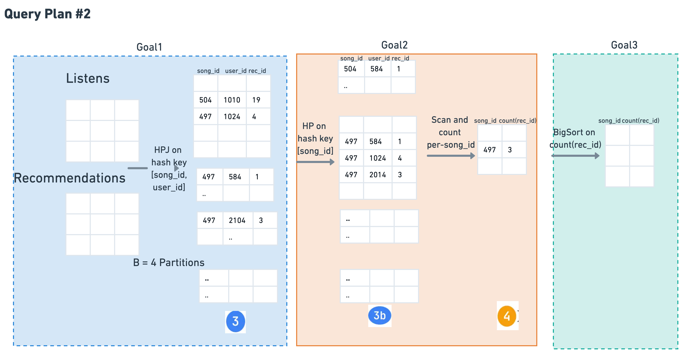
Figure: Plan #2 uses a hash-partition join, which produces unsorted output and requires an extra sort before grouping.
Note. HPJ partitions on [song_id, user_id], so the output partitions (3) are split on both keys. Since GROUP BY is on song_id alone, we must re-partition (3) on song_id to align before grouping. That's the extra HP(3) step.
| Goal | What happens | Cost |
|---|---|---|
#1 Join R, L on [song_id, user_id] |
Hash-Partition Join | HPJ(R, L) |
#2 Group BY song_id |
Re-partition (3) on song_id alone (call it (3b)); read (3b), write (4) |
HP(3) + C_r·P(3b) + C_w·P(4) |
#3 Sort ORDER BY count |
Final sort of (4) |
BigSort(4) |
Total cost (Plan #2): HPJ(R,L) + HP(3) + C_r·P(3b) + C_w·P(4) + BigSort(4)
Why the Plans Differ
| Plan | Key property | Trade-off |
|---|---|---|
| Plan #1 (SMJ) | SMJ output is naturally sorted on the join keys; song_id is a prefix → can group directly |
Pays the sort cost upfront via BigSort inside SMJ |
| Plan #2 (HPJ) | HPJ partitions on the join keys but GROUP BY needs only song_id → extra repartition step |
Cheaper join when nothing is sorted, but pays repartitioning later |
Both plans need a final BigSort for ORDER BY count. That's unavoidable because the output of grouping is in (song_id, count) order, not count order.
When to pick which
| Choose SMJ when… | Choose HPJ when… |
|---|---|
| Data is pre-sorted or easily sortable | Data is unsorted and very large |
| Memory holds sort buffers | Hash partitioning is more efficient |
Join keys align with GROUP BY keys |
You can absorb the repartition cost |
Next: Reading What a Real Optimizer Chose
So far we've estimated costs ourselves by writing out formulas. In practice, real databases do this work for you and show you the result via the EXPLAIN command. The Reading PostgreSQL EXPLAIN page takes the same cost-formula vocabulary and applies it the other way around: it decodes what plan a real optimizer picked, plus an interactive Colab for exploring plans.