Reading PostgreSQL EXPLAIN
Concept. EXPLAIN shows the physical plan a real optimizer chose for a query: every operator, every cost estimate, every row count, read bottom-up. Mapping each operator back to our cost formulas turns a 10-line EXPLAIN dump into a quick mental check of whether the plan makes sense.
Intuition. When PostgreSQL says Hash Join (cost=12.34..55.24 rows=1000), that's just our HPJ(R, S) with the optimizer's estimate of total work and output cardinality. The same vocabulary you used to compare Plan #1 vs Plan #2 by hand applies. The only difference is that now the optimizer is doing the picking.
In IO Cost Summary you wrote cost formulas by hand to compare two plans. Here you'll go the other way: take a query through PostgreSQL's EXPLAIN, then read its operators back in the same cost-formula vocabulary.
Interactive Query Explainer
Run any SQL through a side-by-side cost calculator and see how the plan changes when you tweak page counts: Colab for Query Optimizer.
Worked Example: What PostgreSQL Chose
Same shape as the queries on the previous page, swapped tables:
-- Popular songs based on number of listens
SELECT Songs.title, Songs.artist, COUNT(Listens.song_id) AS popular
FROM Songs
JOIN Listens ON Songs.song_id = Listens.song_id
GROUP BY Songs.title, Songs.artist
ORDER BY COUNT(Listens.song_id) DESC
LIMIT 10;
EXPLAIN output
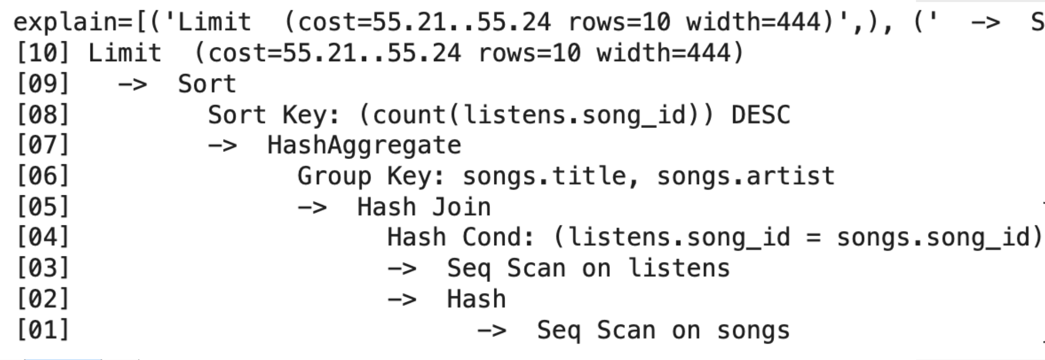
Figure: PostgreSQL's EXPLAIN output for the popular-songs query, showing the plan it picked, estimated cost, and actual row counts at each step.
How to Read EXPLAIN
EXPLAIN is read bottom-up. Leaves are scanned first, and results bubble up to the root.
| Format | Meaning |
|---|---|
cost=startup..total |
startup = cost before first row · total = cost for all rows |
rows=N |
estimated row count flowing out of this step |
Step-by-step on this plan:
-
[01]Seq Scan on songs:C_r × P(Songs)to read the base table. -
[02-03]Build Hash + Seq Scan listens:C_r × P(Listens)to read the second table. -
[04-05]Hash Join:HPJ(Songs, Listens)onsong_id. -
[06-07]HashAggregate: group BY without sorting (in-memory hash table). -
[08-09]Sort:BigSortforORDER BY count. -
[10]Limit: negligible, just take the top 10.
Mapping EXPLAIN → our IO cost formulas
| PostgreSQL operation | Our formula | Cost role |
|---|---|---|
Seq Scan (×2) |
C_r·P(Songs) + C_r·P(Listens) |
base scans |
Hash Join |
HPJ(Songs, Listens) |
join cost |
HashAggregate |
~C_r·P(input) (no sort needed) |
aggregation |
Sort |
BigSort(grouped_data) |
final ORDER BY |
| Total | sum of the above | 55.24 units |
HashAggregate vs. our model. Our simplified IO model assumes grouping requires sorting. Real optimizers also have HashAggregate: build an in-memory hash table keyed by group, accumulate counts, emit one row per group. Cost: C_r·P(input), no sort. If the table doesn't fit in RAM, it spills to disk and falls back to a partition-based approach (essentially HPJ-style).
Why PostgreSQL chose this plan
-
Hash Join beat SMJ because the inputs aren't pre-sorted.
-
HashAggregate beat sort-based grouping because the output (one row per
(title, artist)) fits in memory. -
One BigSort only, for the final
ORDER BY count, not for grouping. -
Total estimated 55.24. The optimizer searched alternatives and this was the cheapest.
The lesson: real optimizers have more tricks than our simplified model, and HashAggregate is the most common one to know about.
Common EXPLAIN Operations Reference
| Operation | What it does | IO cost | Output rows | Output size |
|---|---|---|---|---|
| Sort | Order rows | BigSort cost |
same as input | = input |
| WindowAgg | ROW_NUMBER, RANK, etc. |
C_r·P(input) + sort |
same as input | slightly larger |
| CTE Scan | Reads WITH result |
C_r·P(CTE) |
= CTE rows | = CTE size |
| Subquery Scan | Reads subquery output | C_r·P(subquery) |
= subquery rows | = subquery size |
| Index Scan | Uses index | log(N) + matched rows |
filtered rows | ≪ input |
| Hash Join | Build hash, probe | P(R) + P(S) |
join matches | varies |
| HashAggregate | Group via hash table | C_r·P(input) |
one per group | ≪ input |
| Materialize | Cache result in memory | C_w + n·C_r |
same as input | = input |
Next: Distributed Query Planning extends the same cost-based reasoning across many machines, where shuffle (network hash partitioning) becomes the dominant cost.